Injection Molding Simulation Prediction vs. Actual
Sponsored ContentSimulations have come a long way in the last three decades, but if we seek to prevent dimensional variation, we must understand what provides the highest level of accuracy so we can make good injection mold engineering decisions.
Share
Read Next
With technology today, there are very few reasons we shouldn’t be able to predict with some degree of accuracy the outcome of nearly anything. For injection molded parts, we want to get an inside look before we ever cut steel.
Why? Let’s face it, once the steel chips start to fly, nearly everyone is gun shy about making a change due to the cost and time to do so. But who wouldn’t want to improve design and material selection to prevent dimensional and cosmetic issues while saving money over time?
Simulations have come a long way in the last three decades, but if we seek to prevent dimensional variation, we must understand what provides the highest level of accuracy so we can make good engineering decisions.
The accuracy of simulation is based on 7 factors:
- Mesh
- Algorithms
- Material Characterization
- Mold Design
- Molding Machine
- Processing and User
- Analysis Type
Let’s review each of these 7 factors and see just how close we can get reality to match simulation.
1. Mesh
First, we must define what meshing is and how it works. An easy way to describe this would be by tossing a 1" × 1" × 1" cube into the simulation software and performing the algorithms on just a single entity.
The inherit issue with this is that the cube hasn’t been split into small enough pieces to provide a high level of accuracy. To improve accuracy, we must chop the cube into smaller pieces. When we separate the cube into smaller pieces (shown in Figure 1), we can dramatically increase our accuracy, since the software is now performing calculations on 27 individual components rather than a single entity.

Figure 1: Example of higher mesh count.
When creating a mesh, there is a balance between accuracy and the time the computer requires to perform the computations. In most cases, 500,000 mesh elements can provide results in several hours while 12,000,000 elements can take nearly 36 hours to complete.
Below, in Figure 2, the Design Pod simulation iteration ran in 6 hours. Just keep in mind the computation time is based on available CPU’s and with cloud computing, these values can be dramatically reduced.

Figure 2: Design Pod with 1.5 million elements. Small radii or fillets can be omitted, but it’s crucial to model all the features within the part to ensure that short shots do not occur in snaps or threads.
Figure 3 shows layers within the thickness of the design pod. These are critical to achieve higher accuracy within the simulation, which prevents dimensional change during the cooling process.
Temperatures of plastic drop rapidly due to direct contact with a cold mold during production. Skin layers of the molded part form very quickly, and heat transfer rates change dramatically with the thickness of the skin layer, directly impacting pressure gradients, shrink rates and dimensions, to name a few.
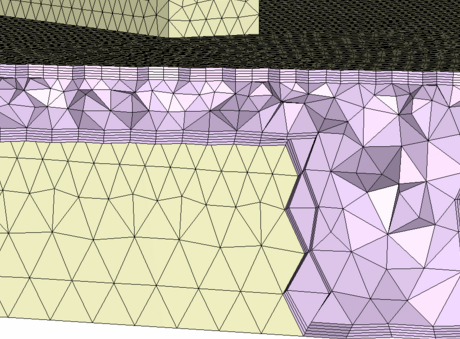
Figure 3: Design Pod with 10 boundary layers (5 per side).
2. Algorithms
Within the software, there are massive amounts of calculations that occur in parallel to provide accurate results. These include (but are not limited to) pressure, temperature and speed. Figure 4 is a relatively simple calculation for cooling that doesn’t take into account all of the variables required for a quality simulation.
Before looking into the equations, we need to first clarify the variables:
- Cp : heat required to raise the temperature of the unit mass of a given substance by a given amount
- λ: ability of material to conduct heat
- ρ: compactness of a substance
- h : wall thickness
- t : time
- T : temperature

Figure 4: Cooling and Thermal Diffusivity Equations
We must remember that there are multiple equations performed on the same element numerous times throughout the analysis. As the part continues to cool, the skin layer becomes thicker and the ability to transfer heat becomes increasingly difficult.
3. Material Characterization
The more that is known about the material behavior under different pressures, velocities, and temperatures, the better the results can be.
There are hundreds of material properties that will impact accuracy and hundreds of thousands of materials on the market. So, it’s not always likely that the material you would be molding is available within the simulation software.
One resource is consulting service TZERO®, designed to ensure good parts from the first shot when launching a new tool, starting with the part design and continuing through production. Generally speaking, when our TZERO® group works on a project, which software we use is heavily weighted on whether or not it has the selected material available.
A fully characterized material is one that has been tested to all the data inputs required by the software package with all the additives included. Without additives like color, slip agents, heat stabilizers, etc., the accuracy can be diminished.
At times, not all the required tests will be performed, and software companies will add generic values from the base family of resins. This is not necessarily a bad practice, but there is a chance results could be skewed high or low.
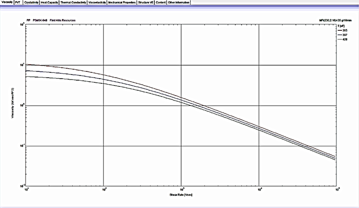
Figure 5: Simulation software material file.
4. Mold Design
Often times, analysts use nodes to represent the gate location, but this has dramatic downsides. It does not fully replicate the flow path the material will take from the molding machine nozzle to the end of the cavity. Using a model like below in Figure 6 that has the full melt delivery system (cold or hot runner), cooling channels, and metal selection is imperative to achieve accuracy.
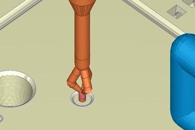
Figure 6: Design Pod with detailed hot drop.
Without the runner system, it’s very difficult to predict pressure loss, which can yield a pressure limited process and parts that shrink more than the shrink rate selected. Missing small details within the hot runner system gate insert geometry can have large negative impacts on the results.
Like most everything else in molding, there is no single rule that applies to everything. There are lots of circumstances where simulations are required, but there is no mold design available. In this scenario, the user must understand mold design and manufacturing well.
5. Molding Machine
The vast majority of molds must work within a certain set of parameters that must be considered when running a proper simulation. In the case of the Design Pod, we needed to collect the variables that impact the mold/machine matching. Once we have the data from each machine, we must design the mold and process for the least capable machine. Table I below shows the limiting machine parameter highlighted in yellow.
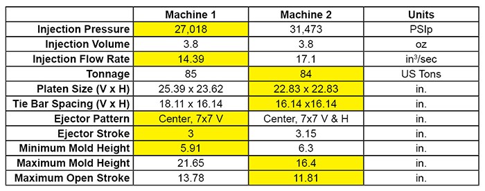
Table 1: Virtual machine capacity comparison showing the limiting machine parameter in yellow.
If an analyst does not take this into consideration, the production facility may not be able to produce parts at the quoted cycle time, scrap rate, or quality criteria needed. This then forces the company to accept lower profit margins or move the mold to a more capable machine, if one exists at their facility with open capacity.
In addition to the molding machine parameter, the simulation user must provide the molder with the flow rates for each circuit to ensure the virtual and real-world replicate each other.
6. Processing and User
The simulation software provides values to plug into the equations, but some of those inputs must be generated by the analyst. Most of the time, the software will default to the average setting for melt and mold temperature, which is great. However, how do we determine the fill speed, hold pressure, etc.?
How fast the cavity should be filled is based on the part quality required at the end. In certain circumstances, like with thin wall parts, the flow rate must be tremendously fast to ensure the cavity is full before the wall freezes. In other instances, like with lens molding, the flow rate must be the complete inverse, almost so that the wall freezes off, but not quite.
This is due to the stress placed on the material during the filling phase. With a lens, we must keep the stress as low as possible to ensure the performance isn’t also impacted. In addition to slow flow rates for lens applications, melt and mold temperatures are typically higher along with hold pressures. These parameters help ensure performance of the lens isn’t negatively impacted.
At times, the software may assist with gate selection. The current software does not take into account the critical to function or process sensitive dimensions that must be tightly controlled and/or monitored. So, the analyst must understand how to interpret drawings and work with marketing to understand where the gate(s) can be placed. On top of that, understanding how cooling can be placed in the mold via standard water passages, baffles, bubblers, or a heat pipe requires extensive knowledge.
In the case of the Design Pod (Figure 7), there were very thin wall sections that dictated that a high flow rate be utilized to ensure the cavity could be filled before the wall froze off and created short shots.
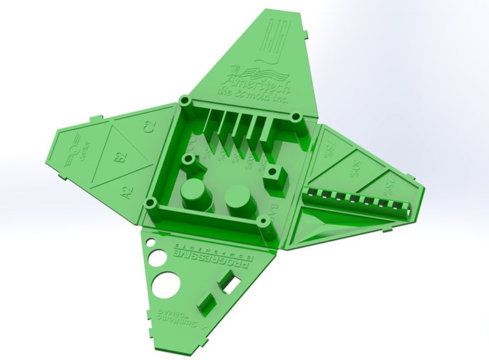
Figure 7: Design Pod with complex geometry.
7. Analysis Types
There are four different types of analyses to run with hundreds of results available for each. Don’t worry, we won’t talk about them all, just some higher-level ones.
The first type is a filling analysis that will show shear heating, shear rates, shear stress, air traps, knit/meld lines, clamp tonnages, and injection pressure to list a few.
Then we have the packing analysis that will provide clamp tonnage, gate seal, potential sinks, and voids.
Cooling helps to determine the overall cycle time based on wall thickness and material section (metal and plastic) as well as cooling line placement.
Warp is inherent to most, if not all, plastic molded parts. It’s just a matter of scale.
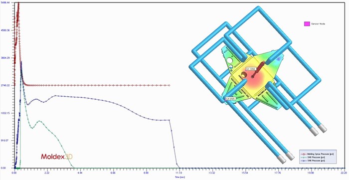
Figure 8: Design Pod cavity pressure predictions.
Template Transfer and Results
Now that we have done our homework and understand everything that goes into accuracy, let’s review the results.
With the simulation packages, RJG has the ability to create a template based on proper sensor location and generate a cavity pressure curve within an eDART® System.
We took inputs from the simulation software and dropped them directly into the molding machine to evaluate predicted vs. reality. In Figure 9 below, we can see the dotted line is the template from simulation, while the solid line is real time cavity pressure curves.
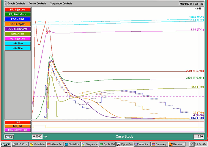
Predicted cavity pressure curves in comparison to actual cavity pressure curves.
The time to fill was within 0.05 seconds of predicted values, and the peak cavity pressure for the end of cavity was off by only 300 PSI. The cooling rate of the actual vs predicted is where simulation still struggles. This reinforces the importance of insuring your algorithms are highly accurate.
Conclusion
Having an intimate understanding of how all 7 of these variables interact with each other can greatly increase the effectiveness and value of a simulation. Be careful not to overlook anything, though, or the simulation report will likely never be seen or heard from again because its final resting place was the circular file.
To learn more about RJG and the eDART® System, click here.
About the Author
Jeremy Williams has over 19 years of experience in the plastics industry serving the medical, automotive, furniture, and appliance industries. He previously worked as a Principal Engineer, taking projects from design concept to sellable products. Jeremy earned his Master Molder II certification in 2011, became an RJG Certified Trainer in 2012, and started at RJG in 2015. In addition to his extensive manufacturing background, he holds degrees in plastics and business. Currently Jeremy is a Consultant/Trainer with TZERO®.

